Failure Analysis
of A Vacuum Tube Guitar Amplifier
EE – 720
Bill Rideout
August 6, 2007
Abstract
This project details a failure analysis of a Gibson Gibsonette vacuum tube guitar amplifier. The goal of this analysis was to determine tests to identify when failure is likely to occur, to develop testing circuitry to perform some of these tests and to develop design modifications to improve the reliability of this amplifier. The modeling program SPICE was utilized to analyze the amplifier circuitry and provide insight into its operation when various components failed. Much effort was expended finding and adjusting SPICE models for the vacuum tubes. While “Design for Testability” focuses primarily on digital integrated circuits, it is hoped that using the SPICE simulator on an analog circuit may shed some insight on the simulation and testing process, or at least identify concerns that might otherwise be overlooked. Finally, an economic analysis of the options developed is presented.
Introduction
Some justification is in order to explain the consideration of vacuum tubes for any application in the twenty first century. Vacuum tube technology has been replaced by solid state electronics in almost all modern applications. Three exceptions for the present and foreseeable future are high power microwave applications, high end audio equipment, and guitar amplifiers. There are several reasons for the use of tubes in guitar amplifiers, some more rational and objective than others. Since the listening experience is ultimately subjective, and depends on the opinion of the listener, one could argue that many claims about the superiority of the sound of tubes are erroneous. However, there are marked differences in the design and operation of tube amplifiers as opposed to solid state amps. A significant factor in the preference for tube amplifiers among guitar players is that when guitars were first being amplified in the 1940’s and 1950’s, tube amplifiers were used exclusively. The sound of the distortion produced by tubes became the hallmark of the amplified guitar sound that remains to this day.
There are many theories and considerations on the difference
between the tube and solid state sound. Vacuum tubes generally progress into
non-linear operation with a ![]() like function while
transistors generally have more of a
like function while
transistors generally have more of a ![]() like function. Also, most tube amplifiers utilize an output
transformer which passes much of the second harmonic and attenuates higher
harmonics. In general, tube amplifiers produce many even harmonics which sound more
consonant to the ear. Transistor amplifiers, which frequently employ negative
feedback to produce a linear output, tend more toward the odd harmonics when
driven into non-linear operation. Conversely, many guitar amplifiers use no
negative feedback. Many contend that tubes have a “warmer” sound and a softer
transition into cutoff. In my humble opinion, this gradual transition into
cutoff is significant. Looking at the output signal of the amplifier used for
this project both on an oscilloscope
and simulated with SPICE, I was impressed with the variation in waveform as the
output tubes were driven further towards cutoff. I also think that tubes just
handle being massively overdriven better that transistors. Of course, modern
DSP technology can mimic tube distortion very well, but many purists will
continue to use tube amplifiers.
like function. Also, most tube amplifiers utilize an output
transformer which passes much of the second harmonic and attenuates higher
harmonics. In general, tube amplifiers produce many even harmonics which sound more
consonant to the ear. Transistor amplifiers, which frequently employ negative
feedback to produce a linear output, tend more toward the odd harmonics when
driven into non-linear operation. Conversely, many guitar amplifiers use no
negative feedback. Many contend that tubes have a “warmer” sound and a softer
transition into cutoff. In my humble opinion, this gradual transition into
cutoff is significant. Looking at the output signal of the amplifier used for
this project both on an oscilloscope
and simulated with SPICE, I was impressed with the variation in waveform as the
output tubes were driven further towards cutoff. I also think that tubes just
handle being massively overdriven better that transistors. Of course, modern
DSP technology can mimic tube distortion very well, but many purists will
continue to use tube amplifiers.
The amplifier I picked for this project is a Gibson model Gibsonette. Although the mainstay of vacuum tube guitar amplifiers were and are produced by Fender, Marshall, and Vox, the electronic circuitry is similar enough that generalizations from the study of the Gibson amplifier should apply to the others as well. I acquired this amplifier in the late 1970’s while in High School. I had to rewire the filter capacitors, apparently someone had tried to replace them and couldn’t figure how to get it back together. I’m guessing that this unit was manufactured sometime in the late 1950’s or early 1960’s. I chose this amplifier because I had access to it and had little qualms about taking it apart for study. Interestingly, there are many guitar players on the web that rave about this little amp, and I’ve read little negative about it. At any rate, it is still in use.
Amplifier Description
From research on the internet, I’ve found that Gibson made several versions of the Gibsonette amplifier. This particular amplifier uses a 12AX7 dual triode for the first and second amplifier stages and two 6V6GT beam power tetrodes in a single ended parallel configuration for the output stage. The vintage schematic found on the internet for this amp is shown in Figure 1. My SPICE schematic is shown in Figure 2.
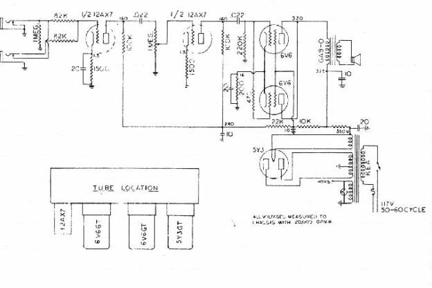
Figure 1. Gibsonette Schematic
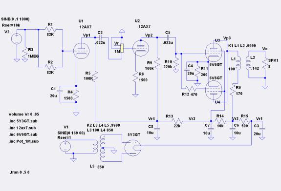
Figure 2. SPICE Schematic
Operation of this circuit is straight forward. The line in Voltage of 169 V is the peak voltage for 120 Vrms. The 5Y3 tube rectifies the 350 Vrms output from the power transformer and supplies the voltage divider ladder made up of R13,R14 and R15. This voltage divider supplies plate voltages for U1, U2, U3 and U4. Note that for SPICE it was convenient to treat U1 and U2 as separate tubes, they are actually both contained in a single 12AX7 tube. For that matter, the U designator was provided by SPICE so I just went with that. Filter capacitors C3, C6, C7, and C8 smooth out the DC voltage and reduce ripple. Cathode resistors R4, R8, and R11 provide a DC voltage at the cathode of U1, U2, U3 and U4 which is positive with respect to the 0 voltage found at the grids. This negative grid voltage biases the tubes into their operating region. Capacitors C1, and C4 provide and ac path to ground so that R4 and R8 to not provide negative feedback. Note that R8 is not bypassed. This version of spice did not have a symbol for a ¼” phone jack so this schematic represents the circuit with an instrument plugged into the top jack of the schematic shown in Figure 1. Resistors R3, R10 and the potentiometer ( R7) provide grid bias resistors.
This amplifier is designed to introduce distortion. The distortion observed at moderate signal levels would make it a terrible choice for a turntable (in keeping with the same era) amplifier. The input signal passes through R1 and/or R2 and is amplified by U1. Typically, very little distortion appears at this stage. With the shown input of 0.1 Vpeak the output at the U1 plate is about 5Vpeak indicating a voltage gain of 50. This signal is fed through coupling capacitor C2 which isolates the DC bias voltage from U1 to U2. The signal passes through the volume control, R7, to the grid of U2. On this schematic, the volume is set at about 2. The volume control potentiometer is described in greater detail in the SPICE section below. Output at the U2 plate at this setting is also about 5Vpeak indicating a unity voltage gain. At volume settings below this point there is actually attenuation in this stage. With an input of 0.1 Vpeak, this stage starts to produce noticeable distortion with the volume control set to about 3. The signal then travels through coupling capacitor C5 to the grids of U3 and U4. Presumably, R12 prevents noise problems that might occur from tying the grids of U3 and U4 together. The plates of U3 and U4 are connected together for a parallel single ended connection that is fed into the output transformer. As a side note, many higher power amps use a push-pull rather than a single ended configuration, but still have two tubes in parallel on each side. With the .1 Vpeak input and volume on 2, the voltage at the input to the output transformer is about 225Vpeak which provides about 8Vpeak on the output side of the transformer. Treating the speaker as a resistive load, the output power is about 4 watts. Noticeable distortion is observed at the output with the volume set at about 2 1/2. R6 is the input winding resistance of the output transformer.
Spice Simulation
Developing the Simulation
I chose Ltspice/SwitcherCAD III version 2.18s for this project. This program is offered free with no restrictions from Linear Technologies. Also, it has very usable schematic creation and schematic capture capabilities. If one wants to use their integrated circuits, it also offers models for their products. Models for passive components such as resistors, capacitors and inductors are provided. However, models for the vacuum tubes had to be developed. Fortunately, this version of spice does provide schematic symbols for both the triode and tetrode. The symbol can be placed in the circuit and then be linked to a sub- circuit for that tube model. I did have to create the symbol for the 5Y3 rectifier.
While considering this project, I searched the internet and found that there are indeed SPICE models that have been created for vacuum tubes. Two excellent sites are http://www.normankoren.com/Audio/Tube_params.html and http://www.duncanamps.com. Mr. Norman Koren has developed phenomenological equations from observed vacuum tube behavior as opposed to strictly applying the conventional Langmuir-Childs law analysis. He has also developed a MATLAB program to determine modeling parameters for specific tubes. I have found references to his work on other sites which lends some credibility to his effort. His model of the 12AX7 works very well and I used it directly in my SPICE simulation. A listing for this device is shown in Listing 1.
Listing 1. 12AX7 SPICE Model
.SUBCKT 12AX7 1 2 3 ; P G C; NEW MODEL (TRIODE)
+ PARAMS: MU=100 EX=1.4 KG1=1060 KP=600 KVB=300 RGI=2000
+ CCG=2.3P CGP=2.4P CCP=.9P ; ADD .7PF TO ADJ PINS, .5 TO OTHERS.
E1 7 0 VALUE=
+{V(1,3)/KP*LOG(1+EXP(KP*(1/MU+V(2,3)/SQRT(KVB+V(1,3)*V(1,3)))))}
RE1 7 0 1G
G1 1 3 VALUE={(PWR(V(7),EX)+PWRS(V(7),EX))/KG1}
RCP 1 3 1G ; TO AVOID FLOATING NODES IN MU-FOLLOWER
C1 2 3 {CCG} ; CATHODE-GRID
C2 2 1 {CGP} ; GRID=PLATE
C3 1 3 {CCP} ; CATHODE-PLATE
D3 5 3 DX ; FOR GRID CURRENT
R1 2 5 {RGI} ; FOR GRID CURRENT
.MODEL DX D(IS=1N RS=1 CJO=10PF TT=1N)
.ENDS
The tetrode model was another matter. While the models I tried accurately modeled gain and biasing of the device, the plate voltages for the 12AX7 were significantly lower than either the measured values from my amp or the values shown on the Gibson schematic. I finally figured out that the reason for this drop in voltage was the effect of the screen current on the voltage divider ladder that supplies the plate voltages to U1 and U2. To explain what was happening necessitated some understanding of the operation of the beam power tetrode. A drawing of a beam power tetrode is shown in Figure 3.
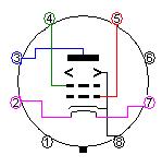
Figure 3. Beam Power Tetrode
(Image from Wikipedia under GNU license)
In this drawing, the screen is attached to pin 4, the plate is attached to pin 3, the grid is attached to pin 5, and the cathode is attached to pin 8. The purpose of the screen is to isolate the electric field of the plate from the electric field of the grid, thereby increasing gain. The screen is normally held at a DC voltage that is slightly less than that of the plate. In a normal tetrode, the screen attracts many of the electrons flowing from the cathode to the plate which results in a large screen current. This current can be up to 80% of the value of the plate current. In the power beam tetrode, the electrons flowing from cathode to plate are focused into a beam by elements that are electrically connected to the cathode. In this way, the effect of the screen on the grid and plate electric fields is still present while the number of electrons actually absorbed by the screen are greatly reduced, therefore dramatically reducing the screen current.
Interestingly, this is not the reason for the invention of the beam power tetrode. A problem with the regular tetrode is that at low signal levels, some electrons bounce off the plate and are absorbed by the screen thereby producing a “knee” in the response. The pentode solves this problem by inserting yet another element, the suppressor grid, between the screen and plate. The beam power tetrode solves this problem by focusing a beam of electrons to prevent electrons from the plate from flowing to the screen. The beam power tetrode was actually invented so that power tubes could be produced that did not violate the patent on the pentode.
The SPICE models that I found for the 6V6 beam power tetrode actually use a pentode model in which has a much higher screen current than the 6V6. This might have gone unnoticed had not this additional current and resulting voltage drop across R14 affected the plate voltages of the 12AX7. I divided the screen current in the 6V6 model by a constant to obtain a more reasonable screen current. The 6V6GT sub circuit model is shown in Listing 2. This model was obtained from the website http://www.audiobanter.com. This model works well for the amplifier simulation.
Listing 2. 6V6GT SPICE Model
*********************
*
* 6V6
* 28 Nov 2004
* new model based on measurements
* parameters revised 29 Nov 2004
*
**********************
..subckt 6V6GT A S G K
XV1 A S G K Pentode2
+ PARAMS: Ex=1.41031468452635 Mug=11.7888046293233 Mus=36.3212284562041
+ Kg1=1084.30402294001 Kp=36.0452435978759
+ Kvb=899.32403046434 Go=-0.467417459629955 Kd=0.000106867654972877
+ Exd=1.26175320982325 Exsd=0.425953018509995
+ C1=-2.85604234699625 A1=-5.68835011136307E-05 B1=3.49035244298882
+ X1=0.015108363529097 Y1=0.00926342558705693 Sr=0.198544592645026
+ Cgk=9P Cgs=5P Cga=0.7P Cak=7.5P
..ends 6V6GT
*******************
*
* Pentode model based on my investigations
* see Excel spreadsheets BeamPentodeModels.xls and Pentode Remote DL
* models.xls
*
* This model is for pentodes with remote cutoff grid characteristics and
* with
* knees that blend into a smooth line, ie a diode line, typical of Beam
* type tubes.
*
* this model therefore uses Korens method for total current, and diode
* lines.
*
* similart to Pentode1, but with revised Capture Ratio formula
*
* default parameters are for the 6V6
*
* RCM 2004 November 28
* 2004 Nov 29 revised capture ratio formula to correct problem when Vg
*> Vp or Vg > Vs
*
************************
..Subckt Pentode2 A S G K
+ Params: Ex=1.42596448566733 Mug=11.7822188645457 Mus=27.5137445137459
+ Kg1=1447.15506010676 Kp=36.3066403677756
+ Kvb=756.918578086785 Go=-0.557407825110845 Kd=0.000103636138847149
+ Exd=1.26335466904983 Exsd=0.431363489073363
+ C1= -0.940657929992395 A1=-0.000127738832949614 B1=1.72299135911867
+ X1=0.0345083152949822 Y1= 0.0177418846473534 Sr=0.0471284218217744
+ Cgk=9P Cgs=5P Cga=0.7P Cak=7.5P
* calculate the total space current based on Koren's triode equations,
* but with an equivalent triode plate volatage equal to the pentode Vs +
*Vp/Mus
En1 n1 0 VALUE={(V(A,K)/Mus+V(S,K))/Kp*LN(1+EXP(Kp*(1/Mug+(V(G,K)-Go)/SQRT(Kvb+(V(A,K)/Mus+V(S,K))**2))))}
Esc sc 0 VALUE={ (PWR(V(n1),Ex)+PWRS(V(n1), Ex))/(Kg1) }
* calculate the plate current capture ratio
Ecr cr 0 Value={If(V(A,K)<=0,0,C1+A1*V(A,K)+B1*((limit(V(A,G),1,1e6)**X1)/(limit(V(S,G),1,1e6)**Y1)))}
* the tentative plate current is total space current multiplied by capture
*ratio
Ept pt 0 Value={V(sc)*V(cr)}
* calculate the diode line current
Ed d 0 value={Kd*V(A,K)**Exd*V(S,K)**Exsd}
* the actual Plate current is the lesser of pt and d
Ep p 0 value={Min(V(d),V(pt))}
Ga A K value={V(p)}
* calculate the screen current capture ratio
* if Vg <= 0 then the screen gets all the remaining current, otherwise the
* grid gets some
Escr scr 0 value={Limit(if(V(G,K)>0,1-Sr*V(G,K),1),0,1)}
* screen current is anything not captured by the plate, multiplied by screen
*capture ratio
Esg sg 0 value={(V(sc)-V(p))*V(scr)}
*Gs S K value={V(sg)}
* Fudge
factor added to reduce screen current in line with observed behavior WFR
7-14-07
Gs S K value={V(sg)/5}
* grid current is anything not captured by the plate or the screen
Gg G K value={V(sc)-v(p)-V(sg)}
* interelectrode capacitances
C1 G K {Cgk}
C2 G S {Cgs}
C3 G A {Cga}
C4 A K {Cak}
..ENDS Pentode2
The potentiometer model adjusts the wiper resistance linearly by varying the reference input voltage from 0 to 1. The model for this sub circuit is shown in Listing 3.
Listing 3. 1M Potentiometer.
* POTENTIOMETER SUBCIRCUIT
*
* TERMINALS: 1-CCW , 2-WIPER, 3-CW
* WIPER POSITION VOLTAGE: 7-POS,8-NEG
*
.SUBCKT POT_1M 1 2 3 7 8
E_RA 1 4 VALUE = { V(7,8) * 1meg * I(VSENSE1) }
VSENSE1 4 5 DC 0V
RS 5 2 1
E_RB 5 6 VALUE = { (1-V(7,8)) * 1meg * I(VSENSE2) }
VSENSE2 6 3 DC 0V
.ENDS
Testing the Simulator
The results of measured voltages and values produced by the SPICE simulation for plates and cathodes at 0V input are shown in Table 1.
|
Plate
Volts |
U1 |
U2 |
U3 |
|
Gibsonette |
155 |
144 |
316 |
|
SPICE |
156 |
156 |
330 |
|
|
|
|
|
|
Cathode
V |
|
|
|
|
Gibsonette |
1.26 |
1.11 |
14.5 |
|
SPICE |
1.1 |
1.1 |
15.2 |
Table 1. Measured and Simulator Voltage
Measuring the output from my Epiphone Dot guitar on an oscilloscope, I found the output voltage at a low volume setting to be about 0.1 Vp-p and the output voltage at the maximum volume setting to be about 0.8 Vp-p. A 1kHz sine wave at 0.1V peak (0.2Vp-p) was used to test and compare the response of the amp to the SPICE simulation. The measured results shown below are cut and pasted from the program Oscillometer 5.60 Demo obtained from http://sbmelyoff.nm.ru . This program uses a computer sound card for its input. I resistively attenuated the signal to protect my soundcard so the voltages shown are not accurate. The voltages observed on an actual oscilloscope are close to those produced by SPICE, however, the primary intent of this comparison is to demonstrate the distortion characteristics. Figures 4 and 5 compare amp and SPICE outputs with R7 set to 25K, corresponding to a volume control setting of about 2. Figures 6 and 7 compare outputs with R7 set to 60K on the amp and 80k on SPICE roughly corresponding to a volume control setting of about 2 1/2. Figures 8 and 9 compare outputs with R7 set to 389K roughly corresponding to a volume control setting of about 5. The output waveforms from the amp itself and SPICE do differ and would not be adequate for other applications, such as developing a DSP simulation. However, they do show a good correlation between the SPICE simulator and the actual operation of the amplifier that can be used to model component failure.
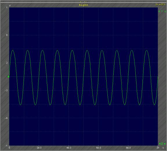
Figure 4. Amp
Output at R7 Wiper to Ground at 25k, Volume at approx. 2
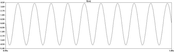
Figure 5. SPICE Output at R7 Wiper to Ground at 25k
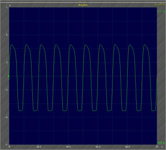
Figure 6. Amp Output at R7 Wiper to Ground at 60k, Volume at approx. 2 ½
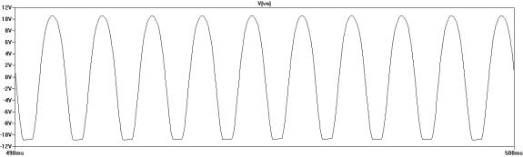
Figure 7. SPICE Output at R7 Wiper to Ground at 80k
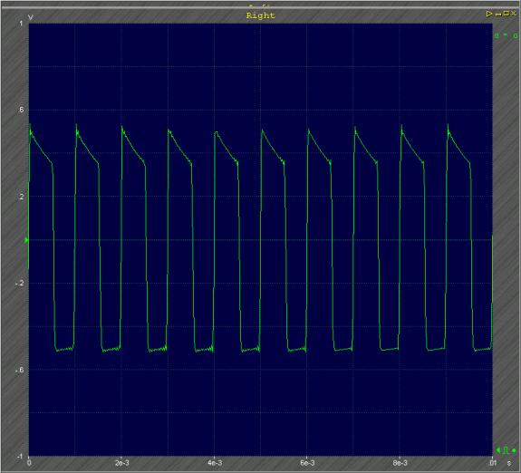
Figure 8. Amp Output at R7 Wiper to Ground at 389k, Volume at approx. 5
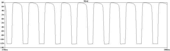
Figure 9. SPICE
Output at R7 Wiper to Ground at 389k
Failure Analysis
Covered Components
This analysis covers failures of resistors, capacitors, vacuum tubes and transformers. Items not covered are the ¼ “ input jacks, fuse, on/off switch and speaker. Failure of these items, while significant, is in large part controlled by how the unit is used or abused and would be difficult to quantify.
Failure Mechanisms
The means by which individual components fail are considered and defined as follows:
Resistors
For this analysis, resistors are considered to fail open. Resistors typically fail as a result of excessive power dissipation which causes them to degrade into an open circuit.
Capacitors
Capacitors can fail open, short, or develop “leaks” which can be modeled by a parallel resistance. Older tube equipment frequently used capacitors made form paper foil and wax. These were prone to leak or short if penetrated by moisture. However, this particular amplifier does not employ these. Aluminum oxide electrolytic capacitors, as used in this equipment, can fail if not used for a very long time as the aluminum oxide requires DC current to maintain its integrity. Also, electrolyte can dry up causing capacitor failure. Capacitors can also fail when their rated voltage is exceeded.
Transformers
Transformers can fail shorted, partly shorted or open. They generally fail when the winding insulation melts or burns as a result of too much current.
Vacuum Tubes
In contrast to other circuit elements, vacuum tubes have a prescribed lifetime and can eventually be counted on too wear out. Typically, as the cathode ages, it will emit fewer and fewer electrons until the tube is unusable. Other methods of failure include shorting of internal elements, and loss of vacuum.
Inductive Failure Analysis
A bottom-up inductive approach was considered to determine the effects of individual component failure. The results are shown in Table 2. Where possible, the SPICE simulator was used to model the results of the failed component.
Component |
Excessive
Current /Power |
No
Amplification |
Low
Amplification |
Ring/Hum |
Noise |
No
Sound |
|
R1 Open |
|
Input 1 |
|
|
|
|
|
R2 Open |
|
Input 2 |
|
|
|
|
|
R3 Open |
|
|
|
|
X |
|
|
R4 Open |
|
X |
|
|
X |
|
|
R5 Open |
|
X |
|
|
|
|
|
R7 Open |
|
X |
|
|
|
|
|
R8 Open |
|
X |
|
|
X |
|
|
R9 Open |
|
X |
|
|
X |
|
|
R10 Open |
|
|
|
|
X |
|
|
R11 Open |
|
X |
|
|
X |
|
|
R12 Open |
|
|
X |
|
X |
|
|
R13 Open |
|
X |
|
|
X |
|
|
R14 Open |
|
X |
|
|
|
|
|
R15 Open |
|
|
|
|
|
X |
|
C1 Open |
|
|
X |
|
|
|
|
C1 Short |
|
X |
|
|
|
|
|
C2 Open |
|
X |
|
|
X |
|
|
C2 Short |
|
|
X |
|
|
|
|
C3 Open |
|
|
|
X |
|
|
|
C3 Short |
T1, U5 |
|
|
|
|
X |
|
C4 Open |
|
|
X |
|
|
|
|
C4 Short |
|
X |
|
|
|
|
|
C5 Open |
|
X |
|
|
|
|
|
C5 Short |
|
|
X |
|
|
|
|
C6 Open |
|
|
|
X |
|
|
|
C6 Short |
R15, U5, T1 |
|
|
|
|
X |
|
C7 Open |
|
|
|
X |
|
|
|
C7 Short |
R4 |
X |
|
|
|
|
|
C8 Open |
|
|
|
X |
|
|
|
C8 Short |
R13 |
X |
|
|
|
|
|
U1 Gain
loss |
|
|
X |
|
X |
|
|
U1 Noise |
|
|
|
|
X |
|
|
U1 Short |
|
X |
|
|
|
|
|
U2 Gain
loss |
|
|
X |
|
X |
|
|
U2 Noise |
|
|
|
|
X |
|
|
U2 Short |
|
X |
|
|
|
|
|
U3 Gain
loss |
|
|
X |
|
|
|
|
U3 Noise |
|
|
|
|
X |
|
|
U3 Sort |
T2.R11,R15,U5,T1 |
X |
|
|
|
|
|
U4 Gain
loss |
|
|
X |
|
|
|
|
U4 Noise |
|
|
|
|
X |
|
|
U4 Short |
T2.R11,R15,U5,T1 |
X |
|
|
|
|
|
U5 Gain
loss |
|
|
X |
X |
X |
|
|
U5 Noisy |
|
|
|
|
X |
|
|
U5 Short |
T1 |
|
|
|
|
X |
|
T1 Open |
|
|
|
|
|
X |
|
T1 Short |
|
|
|
|
|
X |
|
T2 Open |
|
|
|
|
|
X |
|
T2 Short |
U3, U4 |
|
|
|
|
X |
Table 2. Inductive
Failure Analysis
Fault Tree Analysis
The data in table 2 and additional analysis was used to develop two fault trees. Figure 10 shows a fault tree for total failure and Figure 11 shows a fault tree for partial failure.
Qualitative Analysis of the Fault Trees
Qualitative analysis of the fault trees reveal two and conditions, one with the input resistors, and one with the output 6V6GT tubes. Failure of one of these components might yield an amplifier that is partially operational. However, these parts are not redundant and a parts count reliability analysis would not take partial failure into consideration. For the 6V6GT vacuum tubes this is especially problematic because some modes of failure will allow partial operation while some constitute total system failure. I could not find any information on the probability of each type of failure, i.e. low gain (partial failure), or shorted elements (total failure). Another benefit of the fault trees is the graphical representation of noise problems due to capacitor failures.
Quantitative Analysis of the Fault Trees
These fault trees are short trees with many branches. The minimum cut sets, or most all of the cut sets for that matter, identify failure due to the failure of a single component. For this reason, a parts count failure analysis is probably more appropriate. Also, the high failure rate of the vacuum tubes is the controlling factor in a failure analysis.
Figure 10.
Total Failure Fault Tree


 Figure 11.
Partial
Failure Fault Tree
Reliability Calculations
For this analysis, system failure is considered to be any degradation of amplifier performance. Analysis of Table 2 and the circuit schematic yields the conclusion that, for the most part, failure of any single component will cause the amplifier to fail. For this reason, the initial reliability calculations are based on a parts count method. Failure rates for individual components were derived from MIL-HDBK-217F-Notice2.
Initial Calculations
I created spreadsheets to calculate the failure rates of
each component and then calculate the reliability for the amplifier. This
facilitated the ability to immediately see the system sensitivity to de-rating
of an individual component. All spreadsheets are provided in the accompanying
excel file. Table 3 shows the failure rates for each component grouped by
component type. For the resistors and capacitors, the criteria for the failure
rate calculations are shown below the failure rate tables. Note that ![]() represents
represents
failure rate/106.
|
Resistor |
lambda-p |
|
Capacitor |
lambda-p |
|
Tube |
lambda-p |
|
Transformer |
lambda-p |
|
R1 |
0.047703 |
|
C1 |
0.22792 |
|
12AX7 |
70 |
|
T1 |
0.9072 |
|
R2 |
0.047703 |
|
C2 |
0.123728 |
|
6V6GT |
70 |
|
T2 |
1.4256 |
|
R3 |
0.047703 |
|
C3 |
2.97216 |
|
5Y3 |
140 |
|
|
|
|
R4 |
0.119258 |
|
C4 |
1.185184 |
|
|
||||
|
R5 |
0.343834 |
|
C5 |
0.123728 |
|
|
||||
|
R7 |
0.047703 |
|
C6 |
1.42272 |
|
|
||||
|
R8 |
0.119258 |
|
C7 |
0.87552 |
|
|
||||
|
R9 |
0.308669 |
|
C8 |
0.5472 |
|
|
||||
|
R10 |
0.308669 |
|
|
|||||||
|
R11 |
1.142856 |
|
|
|||||||
|
R12 |
0.119258 |
|
|
|||||||
|
R13 |
0.308669 |
|
|
|||||||
|
R14 |
0.78144 |
|
|
|||||||
|
R15 |
1.31328 |
|
|
|||||||
Table 3. Component Failure Rates
Table 4 shows the corresponding reliabilities for a 1000 hour time period.
|
Resistors |
lambda-p |
Reliability |
|
Capacitors |
lambda-p |
Reliability |
|
R1 |
0.047703 |
0.9999523 |
|
C1 |
0.22792 |
0.9997721 |
|
R2 |
0.047703 |
0.9999523 |
|
C2 |
0.123728 |
0.9998763 |
|
R3 |
0.047703 |
0.9999523 |
|
C3 |
2.97216 |
0.9970323 |
|
R4 |
0.119258 |
0.9998807 |
|
C4 |
1.185184 |
0.9988155 |
|
R5 |
0.343834 |
0.9996562 |
|
C5 |
0.123728 |
0.9998763 |
|
R7 |
0.047703 |
0.9999523 |
|
C6 |
1.42272 |
0.9985783 |
|
R8 |
0.119258 |
0.9998807 |
|
C7 |
0.87552 |
0.9991249 |
|
R9 |
0.308669 |
0.9996914 |
|
C8 |
0.5472 |
0.9994529 |
|
R10 |
0.308669 |
0.9996914 |
|
|
|
|
|
R11 |
1.142856 |
0.9988578 |
|
Combined |
|
0.9925497 |
|
R12 |
0.119258 |
0.9998807 |
|
|
||
|
R13 |
0.308669 |
0.9996914 |
|
|
||
|
R14 |
0.78144 |
0.9992189 |
|
|
||
|
R15 |
1.31328 |
0.9986876 |
|
|
||
|
|
|
|
|
|
||
|
Combined |
|
0.9949568 |
|
|
||
|
Tubes |
lambda-p |
Reliability |
|
Transformers |
lambda-p |
Reliability |
|
U1 |
70 |
0.9323938 |
|
T1 |
0.9072 |
0.9990932 |
|
U3 |
70 |
0.9323938 |
|
T2 |
1.4256 |
0.9985754 |
|
U4 |
70 |
0.9323938 |
|
|
|
|
|
U5 |
140 |
0.8693582 |
|
Combined |
|
0.9976699 |
|
|
|
|
|
|
||
|
Combined |
|
0.7046881 |
|
|
||
Table 4. Component
Reliabilities
The total system reliability is:
Design Modifications
Obviously, the failure rate of the vacuum tubes is the dominant reliability problem.
One tube that can be replaced with solid state devices with little or no effect on the quality of sound output is the 5Y3 rectifier tube. According to MIL-HDBK-217F calculations, this tube also has the highest base failure rate.
A circuit that replaces the 5Y3 rectifier with solid state diodes is shown in Figure 12.
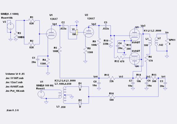
Figure 12. Gibsonette Schematic with Solid State Diodes
Note that an additional series resistor is required since there is much less voltage drop across the solid state diodes than the 5Y3 rectifier tube.
Several other components can be de-rated to improve reliability. Modern aluminum oxide electrolytic capacitors are available with a 600V DC rating. Thus C3, C4, C6, C7 and C8 can be replaced with capacitors with the 600V rating. Replacing the power supply capacitors in an amplifier this old is probably a good idea anyway. These capacitors may very well be leaky and could cause serious damage if they shorted. R11 and R15 can be replaced with 10 watt and 20 watt resistors to improve their reliability.
Table 5 shows the new reliability calculations with the 5Y3 rectifier removed; D1,D2 and R16 added; C3, C4, C6, C7 and C8 replaced; and R11 and R15 replaced.
|
Resistors |
lambda-p |
Reliability |
|
Capacitors |
lambda-p |
Reliability |
|||
|
R1 |
0.047703 |
0.9999523 |
|
C1 |
0.22792 |
0.9997721 |
|||
|
R2 |
0.047703 |
0.9999523 |
|
C2 |
0.123728 |
0.9998763 |
|||
|
R3 |
0.047703 |
0.9999523 |
|
C3 |
0.6912 |
0.999309 |
|||
|
R4 |
0.119258 |
0.9998807 |
|
C4 |
0.250712 |
0.9997493 |
|||
|
R5 |
0.343834 |
0.9996562 |
|
C5 |
0.123728 |
0.9998763 |
|||
|
R7 |
0.047703 |
0.9999523 |
|
C6 |
0.5472 |
0.9994529 |
|||
|
R8 |
0.119258 |
0.9998807 |
|
C7 |
0.5472 |
0.9994529 |
|||
|
R9 |
0.308669 |
0.9996914 |
|
C8 |
0.30096 |
0.9996991 |
|||
|
R10 |
0.308669 |
0.9996914 |
|
|
|
|
|||
|
R11 |
1.015872 |
0.9989846 |
|
Combined |
|
0.9971913 |
|||
|
R12 |
0.119258 |
0.9998807 |
|
|
|||||
|
R13 |
0.308669 |
0.9996914 |
|
Tubes |
lambda-p |
Reliability |
|
||
|
R14 |
0.78144 |
0.9992189 |
|
U1 |
70 |
0.9323938 |
|
||
|
R15 |
1.083456 |
0.9989171 |
|
U3 |
70 |
0.9323938 |
|
||
|
R16 |
1.083456 |
0.9989171 |
|
U4 |
70 |
0.9323938 |
|
||
|
|
|
|
|
|
|
|
|
||
|
Combined |
|
0.994234 |
|
Combined |
|
0.8105842 |
|
||
|
Transformers |
lambda-p |
Reliability |
|
Diode |
lambda-p |
|
|
T1 |
0.9072 |
0.9990932 |
|
D1 |
1.08 |
0.9989206 |
|
T2 |
1.4256 |
0.9985754 |
|
D2 |
1.08 |
0.9989206 |
|
|
|
|
|
|
|
|
|
Combined |
|
0.9976699 |
|
Combined |
|
0.9978423 |
Table 5. Improved Component Reliability
The total system reliability is now:
Testing Circuitry
The failure rate of the vacuum tubes dominate the quantitative failure analysis of the amplifier. Therefore, additional circuitry to identify impending tube failure could alert the user that the tube or tubes need to be replaced, thereby providing a vehicle with which to improve system availability.
Tubes that are wearing out typically have fewer electrons emitted from the cathode. This should decrease the current that flows through the tube in a quiescent state. DC current flowing through the cathode produces a steady biasing voltage seen across the cathode resistor. Monitoring this voltage should give and indication of the aging of the tube. Using the SPICE model, I reduced the gain of the 12AX7’s and 6V6GT’s by 50% and ran a simulation with 0 V input. The voltage on the cathode resistor of the 6V6GT’s went from 15.4V to 6V and the voltage on the 12AX7 cathode resistors went from 1.16V to 0.4V. Also, if elements of the tube were to short out and draw excessive current, this voltage will increase dramatically. Detecting a short or developing short in one of the 6V6GT’s could save the output transformer or filament transformer.
I developed a circuit using a differential amplifier to monitor these voltages. When the voltage is to high or to low, an LED lights. Of course, the LED’s will flash sometimes while the amplifier is being used, but this could be an additional selling point. Figure 12 shows the schematic for the circuit to detect a low voltage condition on the 12AX7 cathode resistors, Figure 14 shows the circuit to detect a high voltage condition on the 12AX7 cathode resistors, and Figure 16 shows the circuit to detect high and low voltages on the 6V6GT’s. V1 is the monitored voltage, and V3 and V4 are 15V voltage regulators. Figures 13,15 and 17 show the response using a SPICE simulation. The straight lines and the scale on the left correspond to the voltage monitored, while the curved line shows the current through the diode.
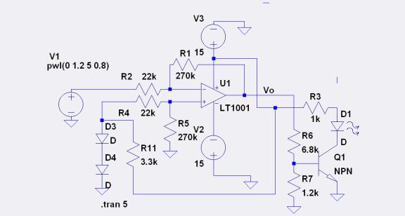
Figure 12. Circuit
to Detect Declining 12AX7 Operation
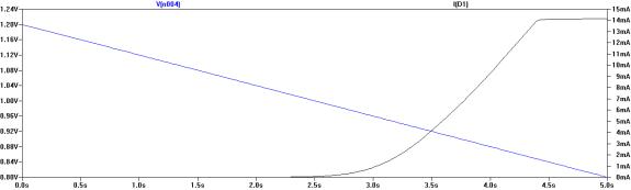
Figure 13. SPICE Simulation of Figure 12 circuit
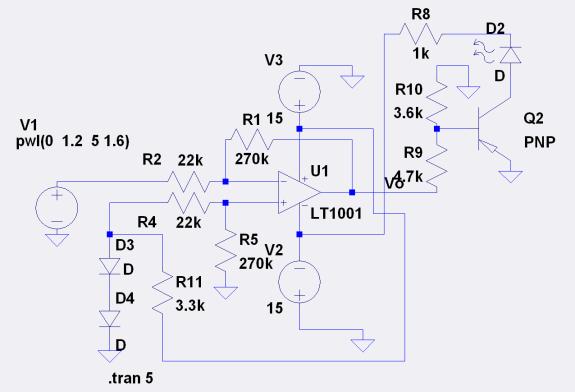
Figure 14. Circuit to Detect 12AX7 Failing Shorted Operation
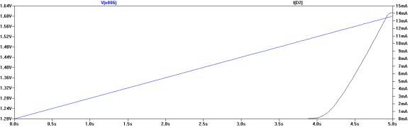
Figure 15. SPICE Simulation of
Figure 14 circuit
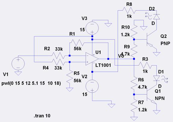
Figure 16. Circuit to Detect Failing and Shorting of 6V6’s
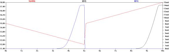
Figure 17. SPICE Simulation of Figure 16 circuit
Financial Considerations
Cost to Maintain Amp With No Design Improvement
Table 6 shows the projected maintenance costs based on reliability for 1000 hours of use. Components are not replaced until they fail. Tube and electrolytic capacitor pricing was obtained from http://thetubestore.com , transformer pricing from http://triodeelectronics.com, and all other components from Digi-Key.
|
Tubes |
lambda-p |
Reliability |
Cost |
Labor |
Per
1000 Hrs |
|
U1 |
70 |
0.9323938 |
$11.95 |
$0.00 |
$0.8365000000 |
|
U3 |
70 |
0.9323938 |
$19.95 |
$0.00 |
$1.3965000000 |
|
U4 |
70 |
0.9323938 |
$19.95 |
$0.00 |
$1.3965000000 |
|
U5 |
140 |
0.8693582 |
$9.95 |
$0.00 |
$1.3930000000 |
|
Total
Tube Cost |
$5.02 |
|
Components |
lambda-p |
Reliability |
Cost |
Labor |
Per
1000 Hrs |
|
||||||||||||||||
|
R1 |
0.047703 |
0.9999523 |
$0.18 |
$40.00 |
$0.0003434642 |
|
||||||||||||||||
|
R2 |
0.047703 |
0.9999523 |
$0.18 |
$40.00 |
$0.0003434642 |
|
||||||||||||||||
|
R3 |
0.047703 |
0.9999523 |
$0.18 |
$40.00 |
$0.0003434642 |
|
||||||||||||||||
|
R4 |
0.119258 |
0.9998807 |
$0.18 |
$40.00 |
$0.0008586605 |
|
||||||||||||||||
|
R5 |
0.343834 |
0.9996562 |
$0.18 |
$40.00 |
$0.0024756019 |
|
||||||||||||||||
|
R7 |
0.047703 |
0.9999523 |
$0.18 |
$40.00 |
$0.0003434642 |
|
||||||||||||||||
|
R8 |
0.119258 |
0.9998807 |
$0.18 |
$40.00 |
$0.0008586605 |
|
||||||||||||||||
|
R9 |
0.308669 |
0.9996914 |
$0.18 |
$40.00 |
$0.0022224154 |
|
||||||||||||||||
|
R10 |
0.308669 |
0.9996914 |
$0.18 |
$40.00 |
$0.0022224154 |
|
||||||||||||||||
|
R11 |
1.142856 |
0.9988578 |
$2.38 |
$40.00 |
$0.1087998912 |
|
||||||||||||||||
|
R12 |
0.119258 |
0.9998807 |
$0.18 |
$40.00 |
$0.0008586605 |
|
||||||||||||||||
|
R13 |
0.308669 |
0.9996914 |
$0.18 |
$40.00 |
$0.0022224154 |
|
||||||||||||||||
|
R14 |
0.78144 |
0.9992189 |
$0.18 |
$40.00 |
$0.0056263680 |
|
||||||||||||||||
|
R15 |
1.31328 |
0.9986876 |
$5.00 |
$40.00 |
$0.2626560000 |
|
||||||||||||||||
|
C1 |
0.22792 |
0.9997721 |
$0.52 |
$40.00 |
$0.0047407360 |
|
|||||||||||||||
|
C2 |
0.123728 |
0.9998763 |
$0.57 |
$40.00 |
$0.0028209984 |
|
|||||||||||||||
|
C3 |
2.97216 |
0.9970323 |
$12.95 |
$40.00 |
$1.5395788800 |
|
|||||||||||||||
|
C4 |
1.185184 |
0.9988155 |
$0.52 |
$40.00 |
$0.0246518272 |
|
|||||||||||||||
|
C5 |
0.123728 |
0.9998763 |
$0.57 |
$40.00 |
$0.0028209984 |
|
|||||||||||||||
|
C6 |
1.42272 |
0.9985783 |
$12.95 |
$40.00 |
$0.7369689600 |
|
|||||||||||||||
|
C7 |
0.87552 |
0.9991249 |
$12.95 |
$40.00 |
$0.4535193600 |
|
|||||||||||||||
|
C8 |
0.5472 |
0.9994529 |
$12.95 |
$40.00 |
$0.2834496000 |
|
|||||||||||||||
|
T1 |
0.9072 |
0.9990932 |
$39.99 |
$40.00 |
$1.4511571200 |
||||||||||||||||
|
T2 |
1.4256 |
0.9985754 |
$59.95 |
$40.00 |
$3.4185888000 |
||||||||||||||||
|
Component
Cost |
$8.31 |
|
|||||||||||||||||||
Total maintenance cost $13.33
Table 6. Maintenance Cost for 1000 Hours of Operation
Cost to Maintain Amp With Design Improvement
Table 7 shows the projected maintenance costs based on reliability for 1000 hours of use. Components are not replaced until they fail.
|
Tubes |
lambda-p |
Reliability |
Cost |
Labor |
Per
Year Hrs |
|
U1 |
70 |
0.93239382 |
$11.95 |
$0.00 |
$0.8365000000 |
|
U3 |
70 |
0.93239382 |
$19.95 |
$0.00 |
$1.3965000000 |
|
U4 |
70 |
0.93239382 |
$19.95 |
$0.00 |
$1.3965000000 |
|
Total
Tube Cost |
$3.63 |
|
Resistors |
lambda-p |
Reliability |
Cost |
Labor |
Per
Year Hrs |
|
||||||||||||||||||||
|
R1 |
0.0477034 |
0.9999523 |
$0.18 |
$40.00 |
$0.0003434642 |
|
||||||||||||||||||||
|
R2 |
0.0477034 |
0.9999523 |
$0.18 |
$40.00 |
$0.0003434642 |
|
||||||||||||||||||||
|
R3 |
0.0477034 |
0.9999523 |
$0.18 |
$40.00 |
$0.0003434642 |
|
||||||||||||||||||||
|
R4 |
0.1192584 |
0.99988075 |
$0.18 |
$40.00 |
$0.0008586605 |
|
||||||||||||||||||||
|
R5 |
0.3438336 |
0.99965623 |
$0.18 |
$40.00 |
$0.0024756019 |
|
||||||||||||||||||||
|
R7 |
0.0477034 |
0.9999523 |
$0.18 |
$40.00 |
$0.0003434642 |
|
||||||||||||||||||||
|
R8 |
0.1192584 |
0.99988075 |
$0.18 |
$40.00 |
$0.0008586605 |
|
||||||||||||||||||||
|
R9 |
0.3086688 |
0.99969138 |
$0.18 |
$40.00 |
$0.0022224154 |
|
||||||||||||||||||||
|
R10 |
0.3086688 |
0.99969138 |
$0.18 |
$40.00 |
$0.0022224154 |
|
||||||||||||||||||||
|
R11 |
1.015872 |
0.99898464 |
$2.38 |
$40.00 |
$0.0967110144 |
|
||||||||||||||||||||
|
R12 |
0.1192584 |
0.99988075 |
$0.18 |
$40.00 |
$0.0008586605 |
|
||||||||||||||||||||
|
R13 |
0.3086688 |
0.99969138 |
$0.18 |
$40.00 |
$0.0022224154 |
|
||||||||||||||||||||
|
R14 |
0.78144 |
0.99921887 |
$0.18 |
$40.00 |
$0.0056263680 |
|
||||||||||||||||||||
|
R15 |
1.083456 |
0.99891713 |
$5.00 |
$40.00 |
$0.2166912000 |
|
||||||||||||||||||||
|
R16 |
1.083456 |
0.99891713 |
$5.00 |
$40.00 |
$0.2166912000 |
|
||||||||||||||||||||
|
C1 |
0.22792 |
0.99977211 |
$0.52 |
$40.00 |
$0.0047407360 |
|
|||||||||||||||||||
|
C2 |
0.123728 |
0.99987628 |
$0.57 |
$40.00 |
$0.0028209984 |
|
|||||||||||||||||||
|
C3 |
0.6912 |
0.99930904 |
$12.95 |
$40.00 |
$0.3580416000 |
|
|||||||||||||||||||
|
C4 |
0.250712 |
0.99974932 |
$0.52 |
$40.00 |
$0.0052148096 |
|
|||||||||||||||||||
|
C5 |
0.123728 |
0.99987628 |
$0.57 |
$40.00 |
$0.0028209984 |
|
|||||||||||||||||||
|
C6 |
0.5472 |
0.99945295 |
$12.95 |
$40.00 |
$0.2834496000 |
|
|||||||||||||||||||
|
C7 |
0.5472 |
0.99945295 |
$12.95 |
$40.00 |
$0.2834496000 |
|
|||||||||||||||||||
|
C8 |
0.30096 |
0.99969909 |
$12.95 |
$40.00 |
$0.1558972800 |
|
|||||||||||||||||||
|
T1 |
0.9072 |
0.99909321 |
$39.99 |
$40.00 |
$1.4511571200 |
|
|||||||||||||||||||
|
T2 |
1.4256 |
0.99857542 |
$59.95 |
$40.00 |
$3.4185888000 |
|
|||||||||||||||||||
|
D1 |
1.08 |
0.99892058 |
$11.97 |
$40.00 |
$0.5171040000 |
||||||||||||||||||||
|
D2 |
1.08 |
0.99892058 |
$11.97 |
$40.00 |
$0.5171040000 |
||||||||||||||||||||
|
Component
Cost |
$7.55 |
Total maintenance cost $11.18.
Table 7.
Maintenance Cost With New Design
Cost of Design Modification
Estimated cost of the design modification is shown in Table 7. The maintenance cost savings for 8760 hours of use due to the design modification is $116.78 - $104.57 = $12.21. The cost saving per hour use is $12.21/8760 = $0.0013428. Dividing this into the cost of the upgrade - $171.26/$0.0013428 = 127,539 hours or 146 years to break even on cost. Clearly the modifications should only be considered to increase reliability.
|
Component |
Cost |
|
R11 |
$5.00 |
|
R15 |
$5.00 |
|
R16 |
$5.00 |
|
C3 |
$12.95 |
|
C4 |
$0.52 |
|
C6 |
$12.95 |
|
C7 |
$12.95 |
|
C8 |
$12.95 |
|
D1 |
$11.97 |
|
D2 |
$11.97 |
|
Labor |
$80.00 |
|
|
|
|
Total |
$171.26 |
Table 8. Cost of Design Modification
Cost of Testing Circuits
Table 9 shows the estimated component and assembly costs for the testing circuits. This does not include development costs.
|
Component |
Quantity |
Price |
Total |
|
LT1001 |
3 |
$2.88 |
$8.64 |
|
NPN BJT |
2 |
$0.42 |
$0.84 |
|
PNP BJT |
2 |
$0.52 |
$1.04 |
|
15V Reg + |
1 |
$1.66 |
$1.66 |
|
15V Reg - |
2 |
$1.82 |
$3.64 |
|
LED |
4 |
$0.28 |
$1.12 |
|
Diode |
4 |
$0.09 |
$0.35 |
|
22k res |
4 |
$0.17 |
$0.68 |
|
270k res |
4 |
$0.17 |
$0.68 |
|
3.3k res |
2 |
$0.17 |
$0.34 |
|
33k res |
2 |
$0.17 |
$0.34 |
|
56k res |
2 |
$0.17 |
$0.34 |
|
1.2k res |
3 |
$0.17 |
$0.51 |
|
4.7k res |
3 |
$0.17 |
$0.51 |
|
1k res |
1 |
$0.17 |
$0.17 |
|
1.2k res |
1 |
$0.17 |
$0.17 |
|
3.6k res |
1 |
$0.17 |
$0.17 |
|
6.8k res |
1 |
$0.17 |
$0.17 |
|
Transform |
1 |
$12.58 |
$12.58 |
|
Bridge
Rec |
1 |
$0.67 |
$0.67 |
|
20u cap |
1 |
$0.25 |
$0.25 |
|
Board |
1 |
$0.70 |
$0.70 |
|
Assembly |
1 |
$20.00 |
$20.00 |
|
|
|
|
|
|
Total |
|
|
$55.57 |
Table 9. Cost of
Testing Circuits
Conclusions
Simulation can be an important tool in failure analysis. Using the SPICE simulation to determine the results of component failure for the Gibsonette amplifier was helpful but had its problems. The vacuum tube models that I obtained worked well for the typical operation of the tube but fell short at the extremes. For example, when the cathode capacitor was shorted, thereby effecting a cathode to grid voltage of 0V, the tubes should have behaved like diodes and only passed one polarity of the signal. The SPICE models continued to pass the whole signal, however. Also, it was hard to simulate open resistors. SPICE, or this version of it anyway, does not allow any node to be disconnected. When I put in a very high resistance, say a Tera Ohm, many times I would get “singular matrix” errors. I did some research on this and found something said to the effect that while doing calculations, the model eventually looks like an open circuit and crashes. Also, noise caused conditions from stray signals in the environment really should be introduced as they do have an effect on the actual amplifier. Also, the waveforms seen on the ocilloscope were close in magnitude to those seen on the SPICE simulator, but differed somewhat in shape as the tube were driven far into cutoff. One factor is that these tubes are very old and may not be operating according to their specifications. The point to all this is that I expended much effort to develop this model and realize that much more work really needs to be done. This gives me an appreciation for the effort that is required to develop any simulator, analog or digital. Also, I think that one should always be mindful of the fact that simulators and testers are tools that may have their imperfections. Another thing that comes to mind is that digital testing extensively presumes stuck at zero or stuck at one faults. This is obviously appropriate for this type of testing, and CMOS technology is well developed and exhibits predictable behavior. However, I wonder if it is not a good idea to keep in mind that these are all circuits, whether analog or digital, and that marginal operation might cause problems not readily identified with digital testing techniques.
Development of the fault tree for this project might well be an example of too much detail and complication. However, I’m not sure how informative it would have been had it been kept at a higher level. I think that it did demonstrate the strength of looking at failures by means quantitative analysis, especially where partial failure are concerned.
Finally, as a reality check, the quantitative fault analysis recommended work on the power supply and replacing the electrolytic capacitors of the amplifier. In general, this is a good idea as these capacitors frequently cause problems as the become leaky or short. Some purists scoff at the idea of replacing the rectifier tube with a solid state device. However, it would make the amplifier more reliable. Plug in solid state replacements are available commercially.
Bibliography
Valve Amplifiers, Morgan Jones, Elsevier Ltd., Oxford, UK. 2003
The Cool Sound of Tubes, Eric Barbour, IEEE Spectrum, August 1998
Practical Reliability Engineering, Fourth Edition, Patrick O’Conner, John Wiley and sons 2006
Testing of Digital Systems, Jha and Gupta, Cambridge University Press, Cambridge, UK. 2003
Fault
Tree Handbook with Aerospace Applications, Dr.
Michael Stamatelatos, NASA 2002
MIL-HDBK-217F Notice 2, US Department of Defense, December 1991
http://www.normankoren.com/Audio/Tube_params.html